How Do Global Wholesale Power Markets Work?
Explore bidding zones, NEMO regimes, day-ahead products, cross-zonal gate closure and operational participation in European balancing platforms.
Why markets at all
Liberalisation — Britain 1990, Norway 1991, California 1996, the first EU directive in 1996 — unbundled vertically integrated utilities into competitive generation and retail wrapped around regulated network monopolies. The welfare case was about incentives: competition disciplines investment and operating costs, rewards innovation, and above all shifts the risk of technology choice and construction mistakes from captive consumers onto private shareholders. Europe added a second, political motive — a single electricity market as continental integration by other means. Everything on this page is machinery built to make that bet pay.
The machinery is shaped by four physical facts that make electricity a commodity like no other: it cannot be stored at scale, so the system must balance at every instant; every line has a transmission limit, beyond which congestion threatens blackout; moving power dissipates 3–5% of it as heat; and flows obey Kirchhoff's laws, not contracts — power takes every parallel path, creating loop flows nobody transacted. Each market design on this page is a different answer to the same question: how much of that physics to put into the price, and how much to handle beside it.
How are electricity markets designed around the world?
Every liberalised power system answers two structural questions: where prices form (one price per zone, or a price at every network node) and who decides dispatch (participants self-scheduling their own portfolios, or an operator co-optimising the whole fleet). The answers are largely independent — Europe pairs zonal pricing with self-scheduling, the US ISOs pair nodal pricing with central dispatch, and hybrids exist on every continent. Switch between the two dimensions to see how differently the same physics gets organised.
Classification represents the predominant wholesale-market architecture. Detailed scheduling arrangements and exceptions are described in each market profile.
| Nodal market (US) | Zonal market (EU) | |
|---|---|---|
| Spot price | Locational marginal price at each transmission node | One market clearing price per bidding zone |
| Market bidding | Centrally dispatched unit bidding including technical constraints | Free portfolio-based bidding with self-dispatch |
| Market operation | ISOs / RTOs (non-profit, federally regulated) | Power exchanges (NEMOs) and TSOs under CACM |
| Real-time balancing | Real-time market re-clearing every five minutes, with virtual bidding between day-ahead and real-time | Balancing organised by TSOs independently of the wholesale market |
| Congestion management | All transmission lines inside the day-ahead optimisation | Cross-zonal congestion inside the coupling; intra-zonal congestion via out-of-market redispatch |
| Non-convexities | Three-part bids with make-whole uplift payments | Block orders under uniform pricing, no side payments |
European Wholesale Power Markets
Bidding zones are the atoms of the European market: inside each zone every trade clears at one price with no internal transmission allocation, while exchanges between zones compete for scarce cross-zonal capacity through the single day-ahead and intraday couplings. A zone’s borders are therefore economic statements about where the grid is assumed strong — which is why drawing, splitting and reviewing them is among the most contested exercises in European market design. Explore each zone’s market geography, exchange landscape and balancing-platform participation below.
US Power Markets
There is no American electricity market. There are seven organised ones, each with its own tariff, its own capacity arrangement and its own regulator of last resort, and a large part of the country with no organised spot market at all. What the seven share is the architecture the zonal/nodal table above summarises: unit-level bidding into a central dispatch, a day-ahead and a real-time market settled against each other, and a price at every node rather than across an area. Select a US market in the map above to read its profile.
Seven markets, and the third of the country outside them
PJM, MISO, ERCOT, SPP, CAISO, NYISO and ISO New England serve roughly two-thirds of American demand between them. The remainder — most of the Southeast, and the West outside California — is still served by vertically integrated utilities that own generation, transmission and supply together, trade bilaterally with their neighbours, and have no spot market to clear against. A European reader should hold that firmly: the comparison everyone draws with "the US market" is a comparison with the organised third of the map, and the rest looks more like Europe before liberalisation than after it.
That gap is closing from the edges rather than the centre. The Western Energy Imbalance Market extended real-time dispatch into utilities that never joined an ISO, and the day-ahead extension followed once the mechanism had been trusted for a decade. SPP is building a competing western offering. Neither requires anybody to give up their utility, which is precisely why both are spreading where a full market never did.
Central dispatch and unit bidding
This is the difference a European trader notices first, and it runs deeper than nodal pricing. In Europe a participant bids a portfolio: a price and a volume, with the decision about which of its plants runs left to the participant. In an American market the participant offers each unit individually, together with its technical parameters — start-up cost, no-load cost, minimum run and down times, ramp rates — and the market operator solves the commitment and dispatch problem centrally.
The consequence is that the operator, not the trader, decides what runs. Security-constrained unit commitment clears the day-ahead market against the network and the units' technical limits; security-constrained economic dispatch re-solves every five minutes in real time. It produces a more physically feasible outcome than portfolio bidding, and it costs something in return: the optimisation is non-convex, so a single clearing price cannot always recover every committed unit's costs, and the difference has to be paid as an out-of-market uplift. Much of the last decade of American price-formation reform — fast-start pricing, extended pricing rules — is an attempt to push more of that uplift back into the price where it can signal something.
Two settlements, and the market that links them
The day-ahead market is financially binding: what clears is bought and sold at the day-ahead price whether or not the plant runs. The real-time market then settles only the deviation from that schedule, at the real-time price. A generator that sold in the day-ahead market and produces nothing buys the shortfall back in real time; a load that consumes more than it bought pays for the difference.
Because both are financial, the two prices can be arbitraged, and American markets allow it explicitly through virtual bidding: purely financial offers that take a position in the day-ahead market with no intention of generating or consuming, closed out in real time. Virtual bidding is what disciplines the day-ahead price towards the expected real-time price, and it is the closest American analogue to the role Europe's intraday market plays. It also generates recurring argument about whether traders are converging the two prices or profiting from a predictable gap between them.
Locational marginal prices and how congestion is hedged
A nodal price is three things added together: the system-wide energy component, a congestion component that reflects the shadow price of every binding transmission constraint at that location, and a loss component. Two nodes either side of a constrained line have different prices, and the difference is the value of transmission between them, computed by the market rather than administered afterwards.
That creates a hedging problem Europe does not have in the same form. If a generator sells forward at a hub but is paid at its own node, the basis between them is a real risk. The answer is a financial transmission right — a contract that pays the holder the congestion difference between two points, auctioned by the operator and funded out of the congestion revenue the market itself collects. The rights market is what makes long-term contracting possible in a system with thousands of prices, and it is the piece most often missing from casual proposals to move Europe to nodal pricing.
Capacity, or deliberately not
This is where the seven markets diverge most sharply, and the divergence is the most useful part of the American experience for European purposes, because it is something close to a controlled experiment. PJM, MISO, NYISO and ISO New England all run centralised capacity markets, and all four have redesigned them repeatedly — over how to accredit intermittent and storage resources, how far ahead to procure, and how to stop the market paying for capacity that does not show up when tested. CAISO does not run a centralised auction at all: it places a resource adequacy obligation on load-serving entities and lets them contract bilaterally to meet it. ERCOT has nothing — an energy-only market in which the scarcity price produced by the operating reserve demand curve is the entire investment signal.
Europe tends to discuss capacity mechanisms as a yes-or-no question about market failure. The American map shows four functioning centralised markets, one decentralised obligation and one deliberate refusal, all inside the same country and the same regulatory tradition, none of which has collapsed. The interesting question is not whether to have one but which failure each design is built to prevent, and what it costs to prevent it.
Who actually writes the rules
An American market changes its rules by filing them. The operator proposes a tariff amendment under section 205 of the Federal Power Act, stakeholders and the market monitor intervene, and the Federal Energy Regulatory Commission accepts or rejects it. That makes a single federal regulator the decision point for six of the seven markets, and it is why a FERC order can change market design across half a continent at once.
ERCOT is the exception that explains the rest. Because it is not synchronously interconnected across state lines, it falls outside federal jurisdiction, and its rules are set by the Public Utility Commission of Texas and ultimately the Texas legislature. That independence is why ERCOT could adopt an energy-only design and a reserve demand curve that no federally regulated market has matched, and it is also why the political response to the 2021 winter failure ran through a state legislature rather than a regulator.
Set against Europe, the contrast is less about centralisation than about where the argument happens. Europe writes network codes that bind every member state and then spends years on national implementation, with ACER arbitrating between regulators who each answer to their own government. The United States argues once, in front of one commission, and lives with the answer. Neither is obviously better; they fail differently, and they fail at different speeds.
What the comparison is worth
The American markets are not a template. They rest on a nodal network model built alongside the market rather than retrofitted to it, on one regulator for six of the seven, and on a tolerance for prices that European regulators would cap long before they were reached. But they are the only place where several European open questions have already been answered in practice at scale — whether reserve can be priced by co-optimisation rather than procured ahead, whether congestion can sit inside the price, and whether an energy-only market can finance capacity — and the answers are visible in operation rather than in modelling.
| Market | Footprint | Capacity arrangement | Design feature worth knowing |
|---|---|---|---|
| PJM | Thirteen mid-Atlantic and midwestern states plus DC | Centralised capacity market, procured years ahead | The largest market by demand, and the most contested capacity design in the country |
| MISO | Fifteen central states and Manitoba | Centralised auction, seasonal since 2023 | A long, thin footprint from the Gulf to Canada, so seasonal and locational adequacy dominate |
| ERCOT | Most of Texas, its own interconnection | None: energy-only | Scarcity priced by an operating reserve demand curve; outside federal jurisdiction |
| SPP | Fourteen states across the central plains | Resource adequacy requirement, not a centralised auction | Highest wind penetration of the seven; extending a market westward |
| CAISO | Most of California, plus a wider real-time and day-ahead footprint | Obligation on load-serving entities, met bilaterally | Runs the imbalance and day-ahead markets that reach utilities outside any ISO |
| NYISO | New York State | Centralised capacity market, procured close to delivery | Severe internal congestion between upstate generation and downstate load |
| ISO New England | Six New England states | Centralised forward capacity market, being reformed towards prompt procurement | Winter fuel security, on a system at the end of the gas pipeline network |
Footprints and arrangements are summarised; each market's own tariff governs. Capacity design in particular is under active reform in several of these markets — see the US monitor for what is moving.
From forward hedging to real time
Two market layers run on very different clocks: financial hedging positions build over years, while the physical spot sequence compresses everything that matters into the final thirty-six hours.
Market structure
European wholesale trading is a relay across time: each market in the sequence hands a more accurate position to the next, and each exists to correct what the previous one could not yet know.
Forward markets
Years to days ahead, futures on exchanges and bilateral contracts — including the fast-growing PPA market — let generators lock revenue and suppliers lock cost. Forward liquidity varies enormously by zone, and its absence is itself a design problem: hedging depth determines who can bear merchant risk.
The hedge is the market's founding product. A retailer selling fixed-price contracts is short electricity it does not yet own; a generator's margin floats with every price move — derivatives let both take a known price now rather than carry the risk. The instruments are standardised to pool liquidity: base contracts (constant power, every hour of the delivery period) and peak contracts (business hours, weekdays), traded as futures and options on exchanges or as forwards and swaps over the counter, for delivery periods from days to years. Most are cash-settled against the average spot price of the period — the day-ahead auction thus prices the entire curve above it — though physical futures that mature into actual delivery schedules also trade in Europe. Maturities stretch to ten years on the liquid hubs, but depth concentrates where hedging needs do: the next three months, three quarters, three years.
Because electricity cannot be stored at scale, the usual no-arbitrage link between futures and spot breaks down: there is no cost-of-carry to anchor the curve, so forward prices reflect only expectations about delivery-period fundamentals and the risk aversion of those trading them. That makes hedging markets thinner and more fragile than in storable commodities, and it is why churn — traded volume over physical consumption, around twelve in Germany, near one in small zones — is watched as a health indicator. Locational risk has its own instruments: physical and financial transmission rights hedge the spread between two zones or nodes. Europe uses both, border by border, auctioned through JAO; the US nodal markets use FTRs only, auctioned by the ISOs, with nodal futures layered on top to manage basis risk down to the settlement point.
| Exchange | Contract | Delivery location | Maturities | Settlement |
|---|---|---|---|---|
| EEX | Futures & options | Bidding zone (e.g. Germany) | Days, weeks, months, quarters, years | Cash-settled vs average spot (physical futures also listed) |
| Nasdaq | Futures | Bidding zone (Nordics) | Months, quarters, years | Cash-settled |
| ICE | PJM Real-Time Western Hub futures | Hub (PJM) | Days, weeks, months, quarters, years | Cash-settled |
| Nodal Exchange | CAISO SP15 day-ahead futures | Transmission node / hub (CAISO) | Days, weeks, months, quarters, years | Cash-settled vs monthly average LMP |
Who trades, and where
Two populations meet in the order book. Fundamental participants — generators selling output, retailers sourcing supply, and increasingly aggregators marketing fleets of small assets — carry positions to delivery; even TSOs trade fundamentally in Europe, buying back their grid losses on the spot market. Speculative participants — trading houses, funds, banks — hold zero net volume at delivery; their role is to take the other side, carry risk between hedgers, and keep prices honest across products and time. The venues split the same way everywhere: exchange trading is anonymous, with a clearing house standing behind every trade — daily margining and collateral convert counterparty risk into a system utility — while over-the-counter trading is bilateral and name-to-name, cheaper for the creditworthy, and increasingly registered for clearing at the exchange anyway. Market makers stitch the two together, contractually quoting two-way prices for the spread and fee rebates — paid liquidity where liquidity will not grow wild.
Day-ahead: the reference price
The single day-ahead coupling (SDAC) clears one pan-European auction at noon: one algorithm (EUPHEMIA) matching orders across all zones while allocating cross-zonal capacity implicitly. Its hourly — increasingly quarter-hourly — clearing prices are the reference for imbalance settlement, PPAs, futures and support schemes alike.
The auction is a welfare maximisation: the algorithm chooses acceptances that maximise consumer surplus plus producer surplus plus congestion revenue across every coupled zone at once. Where cross-zonal capacity suffices, prices converge and the capacity is implicitly free; where a border saturates, a spread remains and spread times flow becomes congestion revenue for the TSOs. The lineage matters: EUPHEMIA evolved from COSMOS, the algorithm built for the 2010 Central Western Europe coupling, and inherited its architecture — a branch-and-bound search over block-order combinations, mid-point rules for resolving price indeterminacy, and quadratic sharing rules that split unavoidable curtailment proportionally across zones when price-taking orders cannot all be served. What looks like a single number at noon is the output of one of the larger optimisation problems run daily anywhere in commerce — hundreds of thousands of orders, cleared in minutes, under rules negotiated to the decimal.
| Format | Double-sided sealed-bid uniform-price auction, one clearing per bidding zone and delivery period |
| Timing | Order books close at 12:00 CET on D−1, every day of the year; results published within the hour; TSO nominations by 14:30 |
| Coupling | Single day-ahead coupling (SDAC) across participating zones; EUPHEMIA allocates cross-zonal capacity implicitly with the energy |
| Products | Delivery periods per market time unit — hourly, transitioning to 15 minutes; quotation in €/MWh |
| Order types | Hourly limit orders (stepwise or interpolated), block orders (regular, profile, linked, exclusive), complex orders in some zones |
| Price bounds | Harmonised floor and cap, deliberately asymmetric, with automatic upward adjustment of the cap after near-cap prices |
| Role of the price | Reference for imbalance settlement, futures cash settlement, PPAs and support schemes; the schedule it produces is physically binding |
Intraday: correcting the forecast
The single intraday coupling (SIDC) runs continuous cross-border trading up to gate closure near delivery, supplemented by intraday auctions (IDAs) that price capacity at discrete moments. As wind and solar shares grow, intraday shifts from an error market to the venue where the real dispatch decisions happen.
The structural driver is forecast error. Between the day-ahead auction and delivery, wind and solar output revises by gigawatts — and the error is not linear: it grows with forecast output and spikes near turbine cut-out speeds, when storms force fleets offline faster than forecasts anticipate. Intraday is where that error is closed out voluntarily before the balancing market closes it expensively. Price behaviour near delivery has a characteristic signature: average levels track day-ahead, but tails fatten — extreme positive and negative prices concentrate in the final hours, which is precisely where flexibility earns its money. Early German evidence made the point starkly: by 2012 a flexible CCGT capturing intraday spreads could earn several times its collapsing day-ahead margin, an early sign that volatility close to delivery, not the day-ahead price level, was becoming the remuneration channel for flexibility.
Liquidity arrived as a snowball. In 2010 most continuous trading happened in the last two hours before gate closure; each design improvement — cross-border coupling, quarter-hourly products, shorter lead times — pulled activity earlier and deepened the book, which attracted more participants, which deepened it further. Today's regime of pan-European continuous trading to minutes before delivery, punctuated by three IDAs that generate reference prices and allocate capacity at discrete moments, is the mature form of that trajectory.
Why intraday has auctions at all
Continuous trading and auctions answer the same question differently. Continuous matching takes orders as they arrive and pairs them one by one; an auction pools every order submitted before a deadline and clears them together at a single price. Europe built its cross-border intraday project around continuous order books, and the CACM guideline permitted either — so the case for adding auctions had to be made empirically. Germany supplied the test: a 15-minute intraday auction was introduced in December 2014 alongside the existing continuous market, letting the two mechanisms be observed side by side in the same bidding zone.
The measured effects ran in one direction. Adding the auction raised liquidity, deepened the book — revealing capacity and flexibility that participants had not been posting continuously — and reduced price volatility. The qualitative case is broader than those three indicators. An auction is a moment at which everyone has to be present, which is what produces a price liquid enough to settle hedging products, and hedging needs grow precisely as renewable shares raise volatility. It defuses the high-frequency arms race that continuous matching rewards, because speed buys nothing when clearing is simultaneous. It consolidates position changes at known times, which helps operational reliability. And it allows cross-zonal capacity to be allocated implicitly and optimally at that instant — flow-based, if the region calculates that way — rather than first-come-first-served, which is the only route by which the scarcity value of intraday transmission acquires a visible price.
Europe answered the question in the affirmative. The three intraday auctions in the clock above went live across single intraday coupling on 13 June 2024, with quarter-hour products and implicit cross-zonal allocation, running alongside continuous trading rather than replacing it. The design questions left open in 2016 are the ones now in play: which bid formats let a plant express its technical constraints without slowing the clearing, multi-part bids being the obvious candidate; how often auctions should run, given that each additional one adds a rebalancing opportunity but divides the liquidity; whether standing orders can combine depth with frequency; and how much cross-zonal capacity an auction should be allowed to take, which turns on how well the system operator can recompute the resulting flows.
Balancing as the backstop price
After intraday gate closure, remaining deviations settle at imbalance prices derived from balancing-energy activations. Because every trader compares expected intraday prices against expected imbalance exposure, balancing design reaches backward to discipline the whole sequence.
Price formation
One clearing price per zone per delivery period — how it forms, what it pays for, and why everyone accepted is paid the same.
Marginal pricing and the energy rent
Marginal pricing sets one clearing price per zone per delivery period — the merit order made into a price, cleared where supply meets demand. Orders range from simple limit bids to block, exclusive and linked orders expressing start-up costs and minimum run times — scarcity, negative prices, intertemporal limits and opportunity costs all shape bids and outcomes. Negative prices are permitted and meaningful — they signal inflexibility and subsidy design more than abundance alone.
The theory runs back to Boiteux: welfare is maximised when price equals the short-run marginal cost of the last plant needed — the merit order made into a price. The gap between that price and each cheaper plant's own marginal cost is the energy rent, and it is not excess profit: it is the only channel through which an energy market repays capital. Long-run equilibrium is precisely the state where the least-earning plant's annual rent just covers its fixed costs — rents persistently above that trigger entry, below it, exit. Every argument about scarcity pricing, price caps and capacity mechanisms is at bottom an argument about whether this rent channel is allowed to work.
The merit order: plants sorted by ascending short-run marginal cost. As demand moves from night to day to peak, the clearing price walks up the staircase — and every plant left of the margin earns the gap between the price and its own cost.
Why one clearing price?
Paying every accepted seller the single clearing price, rather than each its own bid, looks like a gift to inframarginal plants — and calls to switch to pay-as-bid resurface in every price crisis. The case against is not ideological but mechanical. Under uniform pricing, a competitive bidder's dominant strategy is to bid marginal cost: bidding higher risks losing profitable dispatch, lower risks selling at a loss. Under pay-as-bid, that logic collapses — every bidder must instead guess the clearing price, so bids encode forecasting skill rather than costs, cheap plants with optimistic forecasts price themselves out while dearer ones run, and small players who cannot afford forecasting desks are structurally disadvantaged. Experimental and theoretical work finds prices no lower, and market monitoring becomes harder because cost-reflective bids — the monitor's benchmark for spotting withholding — disappear by design. Great Britain's regulator, offered the choice at the 2001 NETA reform, confined pay-as-bid to residual balancing volumes and kept it out of the wholesale auction; Europe's day-ahead design has followed that judgment since.
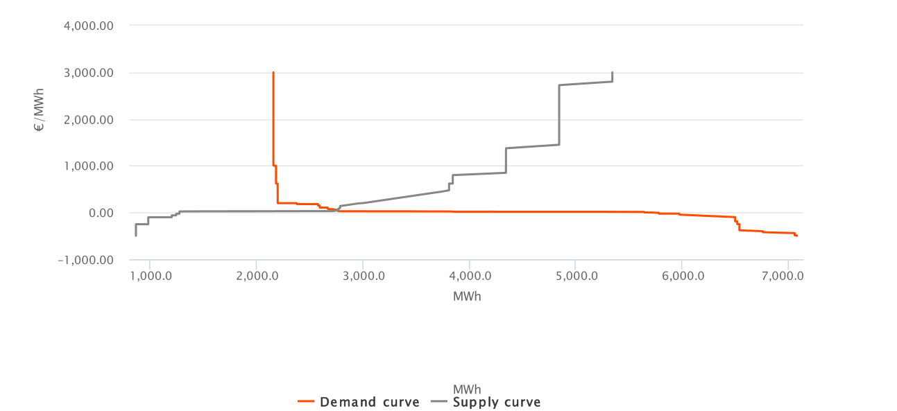
Aggregated day-ahead curves, Austria, 2 June 2020, hour 19–20 (Vassilopoulos & Lahmar 2020, Fig. 9; source: EPEX SPOT). The demand curve is near-vertical — price-inelastic — down to the clearing region, then runs flat toward the floor; the supply curve climbs in steps toward the cap. Every accepted buyer pays, and every accepted seller receives, the price where they cross.
Products: hours, quarter-hours and blocks
The delivery period is the auction’s atom. The 60-minute product is the historical standard — one price per hour, matching the hourly settlement world the markets were born into. The 15-minute product exists because the system stopped varying hourly: solar ramps, imbalance settlement and flexible assets all live at quarter-hour granularity, and pricing them hourly averages away exactly the steepness that flexibility is paid to serve. Germany led with a dedicated 15-minute auction in 2015 to let participants shape their solar ramps; with the market time unit moving to 15 minutes across Europe, the quarter-hour is becoming the atom rather than the exception. Its price profile within each hour reveals what the hourly price conceals — the ramp.
Block orders solve a different problem: a thermal plant’s economics do not decompose into independent periods. Start-up costs and minimum run times mean a plant is only profitable if it runs several consecutive periods — so a block bids them together, all-or-nothing, judged against the volume-weighted average price across its span. Profile blocks vary the volume hour by hour, linked blocks make one block’s acceptance conditional on another’s, exclusive groups let alternatives compete of which at most one clears. The fill-or-kill rule is what makes the auction combinatorial — and what makes paradoxical rejection possible: the price of letting physics into the order book.
Where Europe and the US diverge
Where the designs genuinely diverge is non-convexity and mitigation. Europe folds start-up economics into block orders under one uniform price with no side payments; the US takes three-part bids — start-up, no-load, marginal energy — and pays make-whole uplift outside the price when revenues fall short of offered costs. Mitigation differs the same way: US offer caps are unit-level and cost-justified (PJM's 2,000 $/MWh offer cap with scarcity pricing beyond it) precisely because local market power is visible at nodal granularity, while Europe polices zone-level prices against harmonised technical bounds and leaves conduct to competition authorities.
When prices go negative
A negative price means producers pay to keep producing — and it is rational more often than it sounds. Must-run units stay on because stopping and restarting costs more than a few negative hours; CHP plants owe heat regardless of the power price; units held for reserves must remain synchronised to deliver them. Support schemes add a second layer: a producer paid a premium per megawatt-hour generated loses money by stopping until the price falls below minus the premium, so subsidised fleets rationally bid deeply negative. The result is that negative prices measure inflexibility and subsidy design at least as much as they measure abundance.
That makes them one of the most diagnostic numbers in the system: their frequency tracks the collision between growing must-take renewables and a fleet not yet flexible enough to get out of the way. The cumulated count of negative-price hours per zone — tracked live in ANALYSE — is effectively a running index of that collision, and every storage, demand-response and flexible-retrofit business case feeds on the hours it counts.
Marketing schemes: full market, feed-in tariff, feed-in premium
How a renewable plant is paid decides how it bids, and therefore what the staircase above looks like at its lower end. Under a feed-in tariff the plant does not bid at all: the grid operator takes the output at a fixed price and sells it into the market on the plant's behalf, price-inelastically, because it has to. That volume arrives in the day-ahead auction as must-sell supply at the floor, with no one in the chain who gains from stopping — it is the single largest source of the negative prices the previous section describes, and its operator carries neither forecast error nor imbalance, both of which are socialised through the support levy. Under a feed-in premium, or direct marketing, the plant or its aggregator sells the power itself and becomes balancing responsible: it forecasts, it pays for its imbalances, it must be remotely curtailable, and it receives a premium on top of what it earns. A fixed premium is a fixed bid below zero — the plant keeps producing until the price falls beneath minus the premium, which is why premium-supported fleets rather than tariff fleets set the depth of a negative hour. A sliding premium, topping up to a reference value from a technology-average market price, weakens that incentive but does not remove it, which is why successive rule changes have withheld the premium in stretches of negative prices, tightening in Germany from six consecutive hours to, for new plant, any negative interval at all, and why EU state-aid rules since 2022 pay no support in negative hours. In the full market, whether merchant or hedged through a power purchase agreement, there is no premium and no floor: the plant earns its capture price, bids its true marginal cost of roughly zero, curtails the moment the price goes below it, and lives with the cannibalisation of its own revenue as the fleet grows — unless a pay-as-produced PPA has quietly recreated the tariff's blindness in private. The direction of travel is toward the last column with a hedge attached: the two-way contracts for difference that EU law now requires for new support keep the plant in the market and settle the difference afterwards, and the choice of reference price inside them is where the dispatch incentive is either preserved or lost.
| Full market (merchant or PPA) | Feed-in tariff | Feed-in premium, fixed | Feed-in premium, sliding | |
|---|---|---|---|---|
| Who sells the power | The plant, a trader or the PPA offtaker | The grid operator, on the plant's behalf | The plant or its direct marketer | The plant or its direct marketer |
| Balancing responsibility | The plant's BRP: forecasting and imbalance cost are its own | None: forecast error and imbalance are socialised | The plant's BRP; remote curtailability required | The plant's BRP; remote curtailability required |
| Revenue per MWh | Capture price, hedged or not | Fixed tariff, whatever the price | Market price + fixed premium | Market price + (reference value − average market value) |
| Price risk sits with | The plant, or whoever it has hedged with | Consumers, via the levy | Shared: market on the plant, premium on the payer | Mostly the payer; residual on the plant through the reference design |
| Bid in the auction | Marginal cost, about zero | Price-taking, in effect at the floor | Minus the premium | Near zero, weakly below it |
| At negative prices | Curtails at once (unless a pay-as-produced PPA pays it not to) | Keeps producing; nobody in the chain gains by stopping | Produces until price < −premium; sets the depth of the negative hour | Produces unless the premium is withheld for the interval |
| In scarcity | Earns the full scarcity price | Indifferent; the tariff is the tariff | Earns market price plus premium: a windfall | Support falls to zero as market value rises; windfall above the reference kept |
| Effect on price formation | Elastic supply that withdraws below zero | Inelastic must-sell volume that deepens negative prices | Inelastic down to −premium | Nearly elastic; depends on the withholding rule |
| Cost of capital | Highest without a hedge; PPA-dependent with one | Lowest | Low | Low |
| Typical use | Large projects with corporate offtake; post-support plant | Small rooftop and legacy plant | Legacy schemes; largely superseded | The European default for supported utility-scale plant, converging on two-way CfDs |
Demand response, dynamic pricing and metering
Everything above describes how supply competes to set a price. The other half of a market is missing from most of it, and the omission is structural rather than rhetorical: the demand curve in a wholesale electricity auction is close to vertical, because almost no consumer sees the price at the moment they consume. Retail contracts are fixed for months, meters historically recorded a single monthly total, and the appliance that draws power has no idea what the market is doing. What clears the auction is therefore supply against a quantity, not supply against a willingness to pay — which is why the price at the top of the curve has to be administratively bounded, and why the section that follows exists at all.
Dynamic pricing is the attempt to restore the missing half. Its forms differ in how much risk they move: a time-of-use tariff sets known prices for known blocks and shifts almost nothing onto the consumer; critical-peak pricing adds a small number of expensive hours called in advance; a spot-indexed contract passes the wholesale price through hour by hour and hands the consumer the full volatility of the market. European law has been pushing in that direction for years — larger suppliers must offer a dynamic price contract to any customer with a smart meter — and the 2024 market design reform, notably, pushed back in the other direction at the same time, adding a right to a fixed-price contract after the 2022 crisis demonstrated what full pass-through does to a household that cannot hedge. Both rights now sit in the same instrument, which is an honest acknowledgement that exposure to the spot price is a product some consumers should be able to buy and none should be forced to hold.
Metering is the precondition, and it is where the ambition usually founders. A dynamic price is meaningless unless consumption is measured and settled at the same granularity as the price is set: a quarter-hourly market price against a monthly meter reading is a fiction. The rollouts diverge sharply. France finished Linky at roughly 95% coverage; Germany, whose market design ambitions are as high as anyone’s, had intelligent metering systems on around 3% of metering points in mid-2025 and a legal requirement to reach 90% only by 2032. A country in that position can legislate any dynamic tariff it likes and almost nobody will be able to be billed on it.
What actually responds is automation, not attention. Measured responses to time-varying tariffs are consistently modest where a human has to act and consistently larger where a device acts on the human’s behalf, which is why the demand side is arriving as heat pumps, vehicle chargers and home batteries under algorithmic control rather than as households watching prices. That has two consequences for market design. It makes the demand side an aggregation problem — individually trivial resources reaching the market through a portfolio, which is what the demand-response network code is for. And it makes elasticity a function of equipment stock, so it arrives slowly, unevenly, and roughly a decade behind the policy that assumes it. Until then the top of the supply curve meets something close to a wall, and the market’s answer to scarcity is a number chosen by a regulator.
Scarcity and the cap
At the other extreme, when demand would exceed all available supply, there is no competitive clearing price at all — near-vertical demand never crosses the supply curve. Whatever price appears in those hours is set by an administrator’s cap, a scarcity formula, or someone’s market power; never by competition. That is why the cap machinery matters so much: the harmonised ceiling with automatic upward adjustment exists precisely to keep scarcity priceable without pretending the market can discover the value of lost load on its own. What those scarce hours must pay for — and what happens to investment when they cannot — is the adequacy problem, treated in full on the Adequacy & Capacity Markets page.
What lost load is worth. The value of lost load is the price a consumer would pay to avoid an involuntary interruption, expressed per megawatt-hour not supplied. It is estimated, not observed — from surveys of willingness to pay, from the output a firm loses when the power stops, from the choices households make when offered interruptible contracts — and it varies enormously by who is cut, for how long, and when. Averaged across a system it lands in the thousands to low tens of thousands of euros per megawatt-hour: Great Britain settles imbalances against £6,000/MWh, raised from £3,000 in November 2018; Belgium's scarcity mechanism uses €8,300/MWh; Texas cut its figure from $9,000 to $5,000 after the 2021 crisis. In the EU each member state must now produce a single national estimate on ACER's methodology, and it does more than describe: divided into the cost of new entry, it yields the loss-of-load expectation a system should plan for, so the reliability standard on the adequacy page is VoLL's arithmetic consequence.
Pricing scarcity before it happens. A market that only ever pays VoLL in the hour load is actually shed pays it too rarely to finance anything and too abruptly to be believed. Loss-of-load-probability pricing fixes both by valuing reserves continuously. A megawatt of operating reserve is worth the probability that losing it causes an outage, multiplied by what that outage costs: an adder of LoLP × (VoLL − energy price), where LoLP is read off the distribution of forecast errors and outages as a function of how much reserve remains. The result is an operating reserve demand curve — the figure below — that is near zero with ample reserve, rises steeply as the margin thins, and reaches VoLL at the minimum contingency level, where any further loss means shedding load. Texas has added it to every energy price since 2014; Great Britain reprices reserve at LoLP × VoLL inside its imbalance calculation; Belgium has computed the adder since 2019 and applies it to its imbalance price. Because the adder rides on whatever the energy price is, scarcity value arrives in the price gradually, on the days it is real, without anyone having to bid it — which is exactly what Europe's day-ahead auctions cannot do: there is no adder, so scarcity has to be bid, and bids stop at the cap.
The cap, and why it moves. The single day-ahead coupling clears within harmonised bounds set under CACM. The ceiling has stood at +4,000 €/MWh since May 2022, lifted from the original 3,000 by the automatic rule, which under the 2023 methodology raises it when clearing prices exceed 60% of the cap in at least two market time units on two different days within thirty rolling days, four weeks after the second event. The floor mirrors it: −500 €/MWh from 2017, lowered to −600 from 28 May 2026 after two days in spring 2026 breached 70% of it. The design intent is that the ceiling should never be the thing that binds. But set the numbers side by side and the tension is plain: a cap of 4,000 against VoLL estimates of 6,000 to 10,000 and beyond means that even a perfectly competitive scarce hour cannot pay what the last megawatt-hour is worth. That gap, hour by hour, is the missing money the adequacy page begins from; LoLP pricing closes it from below, capacity mechanisms from outside, and the choice between them is one of the defining decisions of a market's design.
Parts of this page draw on P. Vassilopoulos & E. Lahmar, Wholesale Electricity Markets: From Theory to Practice (Palgrave, 2020) and P. Vassilopoulos & A. Salah Abou El-Enien, The Intraday Paradigm (IHS CERA, 2013).
Congestion management
The grid does not care where bidding-zone borders are drawn. Congestion management is the set of instruments that reconcile a copper-plate market fiction with a constrained physical network.
Market geography
European markets are predominantly zonal: one wholesale price applies inside each bidding zone, while cross-zonal capacity limits exchanges between zones. Nodal designs instead calculate prices at individual network locations.
The zonal price rests on the copper-plate assumption — that the grid inside a zone is strong enough to ignore, so only borders between zones enter the clearing. Every real constraint that assumption hides must then be relieved after the market closes, by switching topology or redispatching plants, and those costs are not in anyone's price: they are socialised across all users of the zone. The nodal design makes the opposite trade — every constraint is in the price by construction, so an LMP map is also a congestion map — at the cost of thousands of prices and the locational risk that comes with them. Each bidding zone is, formally, just one node of a coarser model; the whole debate is about how coarse the model may be before its fictions cost more than its simplicity saves.
The nodal question
Nodal pricing would internalise every constraint into the price itself, eliminating the redispatch layer at the cost of hundreds of prices, locational risk and a central dispatch apparatus. Europe has so far chosen zonal simplicity with growing side-payments; whether that trade-off survives the renewable build-out is the deepest open question in European market design.
The nodal idea — Schweppe's spot pricing, made operational by Hogan — prices each network location at the cost of delivering one more megawatt-hour there, internalising losses, loop flows and congestion. A two-node example carries the whole intuition: with a free line, both nodes price at the cheap generator plus a small loss gross-up; the moment the line saturates, the importing node jumps to its own local generator's cost. The US markets run this at thousands of nodes with central dispatch and three-part bids; Europe's zonal design asserts a copper plate inside each zone and pays the difference through redispatch. Neither is free — the choice is between locational risk priced visibly at every node and congestion costs socialised invisibly across a zone.
The two-node example (after Vassilopoulos & Lahmar 2020, Fig. 5). Unconstrained, both nodes see the cheap generator’s cost plus losses; the moment the line binds, node B’s price jumps to its own local generator — the price difference is the congestion.
Bidding zones as design objects
A zone asserts that its internal grid is strong enough to ignore. When that assertion fails, internal congestion must be managed outside the market — and the bidding-zone review process exists to ask the uncomfortable question of whether borders should move instead.
Capacity calculation
How much trade a border can carry is calculated, not observed. Net transfer capacity (NTC) methods fix bilateral limits; flow-based methods model critical network elements and let the market itself choose which exchanges use scarce grid headroom. Flow-based is standard in the Core region and expanding — the map between physics and market is drawn here.
Implicit allocation
Since market coupling, capacity and energy clear together: power flows from cheap zones to expensive ones until capacity binds, and the price difference across a constrained border is the congestion price. Explicit capacity auctions survive mainly for long-term transmission rights, allocated via JAO.
The 70% obligation
EU law requires TSOs to make at least 70% of critical-element capacity available for cross-zonal trade — a blunt but consequential rule that forces internal congestion to be handled by remedial actions or zone reconfiguration rather than by quietly curtailing the market.
Redispatch and countertrading
What the market cannot see, the TSO must move: paying generators down on the overloaded side and up on the other. Rising redispatch volumes and costs are the measurable symptom of zones outgrowing their grids — and the financing and cost-sharing of these actions is a live design battleground.
Core market-design choices
Beneath the architecture sit parameter choices that look technical and are anything but — each one shifts risk, liquidity or investment incentives somewhere else.
Market time unit
The 15-minute MTU aligns market prices with the granularity at which renewables and imbalances actually vary. Finer time units price flexibility honestly but fragment liquidity per interval — the perennial granularity-versus-liquidity trade.
Gate closure
Every gate — day-ahead noon, intraday cross-zonal closure near delivery — is a compromise between giving traders the latest forecast and giving system operation time to prepare. Moving a gate reallocates responsibility between market and TSO.
Order-type expressiveness
Block and complex orders let physical constraints into the auction; richer order types (the storage-order debate in SDAC) would let batteries express state-of-charge coupling directly. Expressiveness improves dispatch but complicates the clearing algorithm — EUPHEMIA's runtime is a genuine design constraint.
Blocks are Europe's answer to non-convexity: a plant with start-up costs and minimum run times bids hours together, fill-or-kill, judged against the volume-weighted average price. The cost of that honesty is combinatorial — and one of its consequences has a name. A paradoxically rejected block is in the money at the published prices yet rejected, because accepting it would have moved prices against the whole solution; the design tolerates these (while forbidding the reverse, paradoxical acceptance) as the price of keeping uniform pricing without side payments. The US markets solve the same non-convexity the other way: three-part bids for start-up, no-load and marginal cost, with make-whole uplift payments guaranteeing recovery outside the price. One design keeps the price clean and rejects some efficient blocks; the other dispatches efficiently and leaks cost into unpriced uplift — there is no third option that does both.
Price limits
Harmonised technical price bounds exist to protect systems, not to manage politics — and automatic-adjustment rules that raise caps after near-cap prices are designed to keep scarcity priceable. Where caps bind in practice, adequacy signals are silently amputated.
The bounds have their own history: the first CWE coupling harmonised day-ahead limits at ±3,000 €/MWh, while continuous intraday always ran far wider — ±9,999 €/MWh — on the logic that close to delivery, prices must be free to say anything the system needs said. Today's harmonised day-ahead cap ratchets upward automatically when prices approach it, an explicit design commitment that the ceiling should never be the binding constraint on scarcity. The deliberately asymmetric floor keeps negative prices possible without letting them become bottomless.
Liquidity and market making
A price is only as informative as the depth behind it. Auction concentration, continuous-market fragmentation across venues, and market-making obligations determine whether smaller zones produce usable reference prices at all.
Measuring liquidity is itself design-sensitive. Auctions are judged by resiliency — how little a marginal order moves the price; continuous books by bid-ask spreads and depth. But spreads co-move with price levels and seasons, so no fixed threshold defines “liquid” for a non-storable good: a €5 spread means different things at €40 and €120. The deeper regularity is behavioural — liquidity begets liquidity. Sellers demonstrably respond to price signals (more of them appear when spreads make running profitable), each entrant tightens the book, and tighter books recruit the next entrant. Market-making obligations exist to seed exactly that loop where it will not start by itself.
Governance of integration
SDAC and SIDC are run jointly by NEMOs and TSOs under CACM — a standing negotiation among dozens of institutions, with ACER as referee.
Current developments
Bidding-zone reviews, flow-based rollout, 15-minute market time units, intraday auction design and algorithm methodology changes are all live regulatory processes.
Primary sources & references
Harmonised maximum and minimum clearing prices
The in-force HMMCP methodologies for day-ahead and intraday coupling: the bounds, the automatic adjustment rule and the NEMO communication notes that apply it.
Scarcity pricing in Belgium
Elia's operating-reserve-demand-curve adder: LoLP from the imbalance distribution, VoLL of €8,300/MWh, and its application to the imbalance price.
ERCOT report on the ORDC
The canonical implementation: how the operating reserve demand curve is built and calibrated, the minimum contingency level and the value of lost load.
EU Electricity Regulation
Regulation (EU) 2019/943 on the internal market for electricity.
Electricity network codes & guidelines
European Commission overview of the binding EU electricity market and system-operation framework.
EU electricity market integration
ACER monitoring of forward, day-ahead, intraday and balancing market integration.
Electricity market monitoring
ACER monitoring reports, indicators and underlying market evidence.